Correlation Functions¶

Cluster density profiles are closely related to the correlation function

\[\rho(r) = \rho_0(1+\xi_{\rm hm}(r))\]

That is, the average density of halos some distance \(r\) from the center of the halo is proportional to mean density \(\rho_0=\Omega_m\rho_{\rm crit}\) of the universe and the halo-matter correlation function, or the tendency to find matter near halos. This module makes various correlation functions available. The correlation functions for the NFW and Einasto profiles can also be computed directly from the density profiles by inverting the above equation.

Note

By definition \(\int {\rm d}V\ \xi(\vec{r}) = 0\). Almost no analytic correlation function has this built in, however.

NFW Profile¶

The NFW profile (arxiv) is a 3D correaltion function given by:

\[\xi_{\rm nfw}(r) = \frac{\rho_{\rm nfw}(r)}{\Omega_m\rho_{\rm crit}} - 1\]

The free parameters are the cluster mass \(M_\Delta\) and concentration \(c_\Delta = r_\Delta/r_s\). In this module we choose to define the density with respect to the matter background density \(\Omega_m\rho_{\rm crit}\). The scale radius \(r_s\) is given in \(h^{-1}{\rm Mpc}\), however the code uses concentration \(c_\Delta\) as an argument instead. As written, because of the choice of units the only cosmological parameter that needs to be passed in is \(\Omega_m\). The arguments are identical to the density profile.

Note

The correlation functions can use \(\Delta\neq 200\) as an argument: delta=200.

To use this, you would do:

from cluster_toolkit import xi
import numpy as np
radii = np.logspace(-2, 3, 100) #Mpc/h comoving
mass = 1e14 #Msun/h
concentration = 5 #arbitrary
Omega_m = 0.3
xi_nfw = xi.xi_nfw_at_r(radii, mass, concentration, Omega_m)

Einasto Profile¶

The Einasto profile is a 3D density profile given by:

\[\xi_{\rm ein}(r) = \frac{\rho_{\rm ein}}{\Omega_m\rho_{\rm crit}} - 1\]

In this model, the free parameters are the scale radius \(r_s\), \(\alpha\), and the cluster mass \(M_\Delta\). The scale density \(\rho_s\) is calculated internally, or can be passed in instead of mass. This is the same arguments as the density profile. To use this, you would do:

from cluster_toolkit import xi
import numpy as np
radii = np.logspace(-2, 3, 100) #Mpc/h comoving
mass = 1e14 #Msun/h
r_scale = 1.0 #Mpc/h comoving scale radius
alpha = 0.19 #arbitrary; a typical value
Omega_m = 0.3
xi_ein = xi.xi_einasto_at_r(radii, mass, r_scale, alpha , Omega_m)

1-halo vs. 2-halo Terms¶

The NFW and Einasto profiles describe the “1-halo” density of halos, or the density of a halo within its boundary. However, halos tend to be found near other halos, and for this reason the average density of halos should have a 2-halo term. In other words, as you move far from the center of a halo (e.g. past the scale radius or \(r_{200}\) or a splashback radius or any arbitrary boundary) the halo-matter correlation function becomes the “2-halo” term, or the likelihood that one is in a second halo

\[\xi_{\rm hm}(r >> r_s) = \xi_{\rm 2-halo}(r).\]

The two halo term, as detailed below, should be related to the matter density field and a bias. The specific treatment of this is not unanimously agreed upon.

Matter Correlation Function¶

The matter (auto)correlation function describes the average density of matter.

\[\rho_{\rm m}(r) = \rho_0(1+\xi_{\rm mm}(r))\]

By definition it is related to the matter power spectrum by a Fourier transform

\[\xi_{\rm mm}(r) = \frac{1}{2\pi^2}\int_0^\infty {\rm d}k\ k^2 P(k) \frac{\sin kr}{kr}.\]

There is not consensus on what power spectrum to use. Hayashi & White use the linear matter power spectrum, while Zu et al. use the nonlinear matter power spectrum. Anecdotally, the former is generally better for lower mass halos and the latter is better for higher mass halos. Regardless of what you use, to call this you would do

from cluster_toolkit import xi
import numpy as np
radii = np.logspace(-2, 3, 100) #Mpc/h comoving
#Assume that k and P come from somewhere, e.g. CAMB or CLASS
xi_mm = xi.xi_mm_at_r(radii, k, P)

2-halo Correlation Function¶

Halos are biased tracers of the matter density field, meaning the 2-halo correlation function is

\[\xi_{\rm 2-halo}(r,M) = b(M)\xi_{\rm mm}(r)\]

The bias is described in more detail in the bias section of this documentation (in progress). To calculate the 2-halo term you would do

from cluster_toolkit import xi
from cluster_toolkit import bias
import numpy as np
radii = np.logspace(-2, 3, 100) #Mpc/h comoving
mass = 1e14 #Msun/h
Omega_m = 0.3
#Assume that k and P come from somewhere, e.g. CAMB or CLASS
xi_mm = xi.xi_mm_at_r(radii, k, P)
#Assume that k and P_linear came from somewhere, e.g. CAMB or CLASS
bias = bias.bias_at_M(mass, k, P_linear, Omega_m)
xi_2halo = xi.xi_2halo(bias, xi_mm)

Halo-matter Correlation Function¶

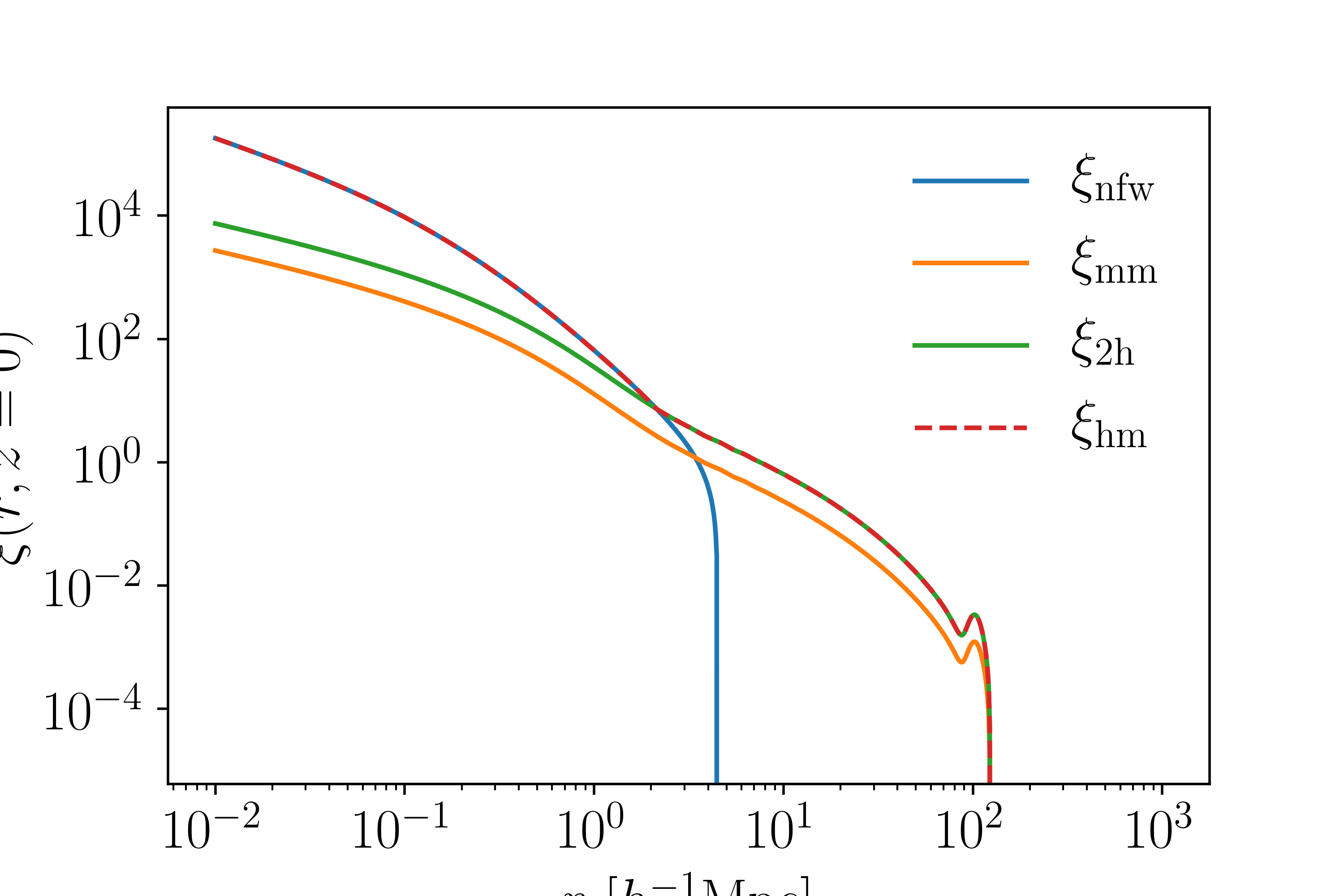
At small scales, the correlation function follows the 1-halo term (e.g. NFW or Einasto) while at large scales it follows the 2-halo term. There is no consensus on how to combine the two. Zu et al. take the max of the two terms, while Chang et al. sum the two. The default behavior of this module is to follow Zu et al., and in the near future it will be easy to switch between different options. Mathematically this is

\[\xi_{\rm hm}(r,M) = \max(\xi_{\rm 1-halo},\xi_{\rm 2-halo}).\]

To use this you would do

from cluster_toolkit import xi
#Calculate 1-halo and 2-halo terms here
xi_hm = xi.xi_hm(xi_1halo, xi_2halo)

Here are each of these correlation functions plotted together: